Introduction to Numpy
This tutorial introduces numpy, a Python library for performing numerical computations in Python.


import numpy as np
np.add(1,1)
Tip: To access the documentation explaining how a function is used, its input parameters and output format we can press
Shift+Tab after the function name"
np.add
a = np.add(2,3)
a
from check_answer import check_answer

# Substitute the ? symbols by the correct expressions and values
answ = ?

check_answer("1.1", answ)
np.array([1,2,3,4,5,6,7,8,9])
arr1 = np.array([1,2,3,4])
arr2 = np.array([3,4,5,6])

np.add(arr1, arr2)
arr1 + arr2
arr = np.array([0,1,2,3,4,5,6,7,8,9,10,11,12,13,14,15])

print(arr[5])
print(arr[5:])
print(arr[:5])
print(arr[::2])
# Substitute the ? symbols by the correct expressions and values
arr = ?
answ = arr[?:?]

check_answer("1.2", answ)
arr = np.array([0,1,2,3,4,5,6,7,8,9,10,11,12,13,14,15])

arr[-2:]
# Substitute the ? symbols by the correct expressions and values
answ = arr[?]

check_answer("1.3", answ)
answ = arr[?:?:?]

check_answer("1.4", answ)
np.array([[1,2,3,4,5,6,7,8,9]])
arr1 = np.array([1,2,3,4,5,6,7,8,9])
arr2 = np.array([[1,2,3,4,5,6,7,8,9]])
arr3 = np.array([[1],[2],[3],[4],[5],[6],[7],[8],[9]])
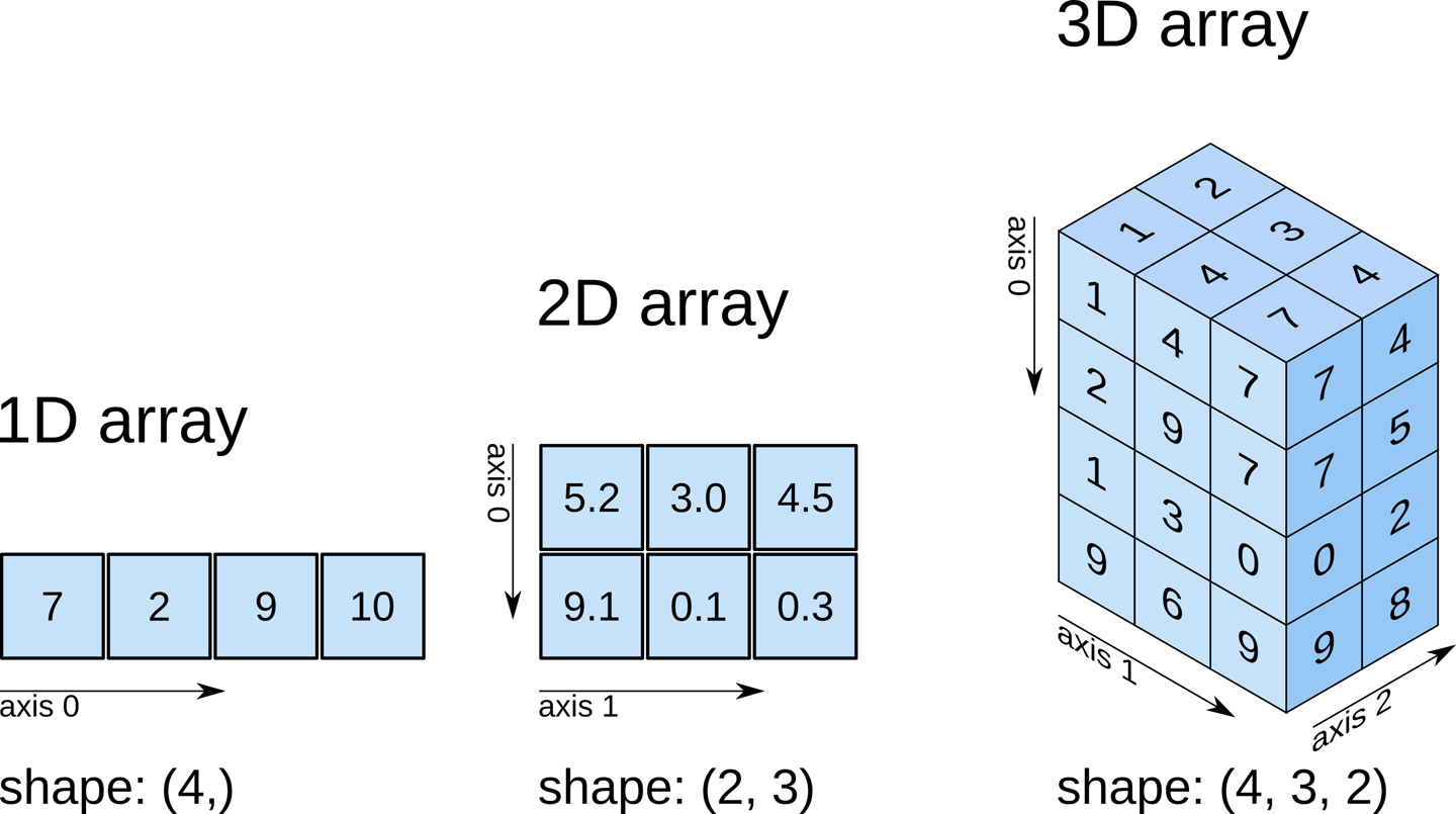
arr1.shape, arr2.shape, arr3.shape, np.array([1,2,3]).shape
np.array([1,2,3,4,5,6,7,8]).reshape((2,4))
See the following example how a 9-element array can be reshaped into two dimensional arrays with different shapes.
Note: We are declaring the array and reshaping all in one line. This is called ’chaining’ and allows us to conveniently perform multiple operations. The expressions are evaluated from left to right, so in this case first we create and array and then apply the reshape operation to the resulting array.
arr1 = np.array([1,2,3,4,5,6,7,8,9]).reshape(1,9)
arr2 = np.array([1,2,3,4,5,6,7,8,9]).reshape(9,1)
arr3 = np.array([1,2,3,4,5,6,7,8,9]).reshape(3,3)

arr1.shape, arr2.shape, arr3.shape
# variable answ should contain your 2-dimensional array with shape (2,3)
answ = ?

check_answer("1.5", answ.shape)
arr1 = np.arange(9)
arr2 = np.ones((3,3))
arr3 = np.zeros((2,2,2))

print(arr1)
print("--------")
print(arr2)
print("--------")
print(arr3)
# variable answ should contain your 3-dimensional array with shape (5,3,3)
answ = ?

check_answer("1.6", answ.shape)
arr1 = ?
arr2 = ?

answ = np.?

check_answer("1.7", answ.shape)
arr = np.arange(9).reshape((3,3))

print(arr)
print("--------")
print("Mean:", np.mean(arr))
print("Std Dev:", np.std(arr))
print("Sum:",np.sum(arr))
arr = np.arange(9).reshape((3,3))

print(arr)
print("--------")
print("Sum along the vertical axis:", np.sum(arr, axis=0))
print("--------")
print("Sum along the horizontal axis:", np.sum(arr, axis=1))
# variable answ should contain your 3-dimensional array with shape (5,3,3)
answ = ?

check_answer("1.8", answ)
Numpy arrays can contain numerical values of different types. These types can be divided in these groups:
- Integers
- Unsigned
- 8 bits:
uint8 - 16 bits:
uint16 - 32 bits:
uint32 - 64 bits:
uint64
- 8 bits:
- Signed
- 8 bits:
int8 - 16 bits:
int16 - 32 bits:
int32 - 64 bits:
int64
- 8 bits:
- Unsigned
- Floats
- 32 bits:
float32 - 64 bits:
float64
- 32 bits:
We can look up the type of an array by using the .dtype suffix.
arr = np.ones((10,10,10))

arr.dtype
arr = np.ones((10,10,10), dtype=np.uint8)

arr.dtype
arr = np.ones((10,10,10))
arr = arr.astype(np.float32)

# Or all in one line
arr = np.ones((10,10,10)).astype(np.float32)

arr.dtype
answ = np.arange(10)

answ = answ#Your code goes here

check_answer("1.9", answ.dtype)
a = np.zeros((10,10))

a = a + 1

a
The previous operation declares a 10x10 array, assigns that to a variable a and then we add 1 to this variable. However, 1 is a single value and is not even an array so it is not entirely clear what is going on. Broadcasting is the ability in numpy to arrays to replicate or promoted arrays involved in operations to match their shapes.
a = np.arange(9).reshape((3,3))

b = np.arange(3)

a + b
Exercise 1.10: Can you declare a new 1-dimensional array with shape (10,) all filled with 2 values?
Tip: We have just seen an example of broadcasting by adding a single value to an array. Broadcasting also works with other operations, such as multiplication or division, so you can complete this exercise declaring an initial array containing all zeros or ones and then using one operation to modify all its values.
answ = ?

check_answer("1.10", answ)
arr = np.array([True, False, True])

arr, arr.shape, arr.dtype
arr1 = np.array([True, True, False, False])
arr2 = np.array([True, False, True, False])

print(np.logical_and(arr1, arr2))
print(np.logical_or(arr1, arr2))
These operations are conveniently offered by numpy with the * and +.
Note: Here the
* and + symbols are not performing multiplication and addition as with numerical arrays. Numpy detects the type of the arrays involved in the operation and changes the behaviour of these operators. This ability to change the behaviour of operators depending on the situation is called ’operator overloading’ in programming languages.
print(arr1 * arr2)
print(arr1 + arr2)
Boolean arrays are often the result of comparing a numerical arrays with certain values. This is sometimes useful to detect values that are equal, below or above a number in a numpy array. For example, is we want to know which values in an array are equal to 1 and the values that are greater than 2 we can do:
arr = np.array([1, 3, 5, 1, 6, 3, 1, 5, 7, 1])

print(arr == 1)
print(arr > 2)
arr = np.array([1, 3, 5, 1, 6, 3, 1, 5, 7, 1])

answ = ?

check_answer("1.11", answ)
arr = np.array([1,2,3,4,5,6,7,8,9])
mask = np.array([True,False,True,False,True,False,True,False,True])

arr[mask]
arr = np.array([1, 3, 5, 1, 6, 3, 1, 5, 7, 1])

answ = ?

check_answer("1.12", answ)
a = np.array([0,0,0])

# We make a copy of array a with name b
b = a

# We modify the first element of b
b[0] = 1

print(a)
print(b)
a = np.array([0,0,0])

# We explicitly make a copy of array a with name b
b = np.copy(a)

# We modify the first element of b
b[0] = 1

print(a)
print(b)